Singular Value Decomposition (SVD)

Data-driven generalization of the Fourier Fransform.

• Singular Value Decomposition - Steve Brunton
• Barry Van Veen: The Singular Value Decomposition - Barry Van Veen
• 7. Eckart-Young: The Closest Rank k Matrix to A - Gilbert Strang
• CS168: The Modern Algorithmic Toolbox

One of the most well used, general purpose tool in numerical linear algebra for data processing. We can use SVD as a data dimensionality reduction tool. SVD allows us to reduce high dimensional data (e.g. megapixel images) into the key features (correlation) that are necessary for analyzing and describing this data.

We can use SVD to solve a matrix system of equations (linear regression models). For example, I have health data for a bunch of patients, we can build a model of how different risk factors map to some disease, we can build the best fit model \(x\) given data \(A\) and \(B\) using least squares linear regression.

SVD is present in:

• image compression / matrix approximation
• recommender system, the Netflix Prize
• linear regression
• PCA (principal component analyzis)
• Google page rank algorithm
• facial recognition algorithm

The SVD allows us to tailor a coordinate system (transformation) based on the data that we have to our specific problem.

matrix decomposition based on simple linear algebra, interpretable features and it’s scalable

Mathematical Overview

hierarchically organized features based on the singular values

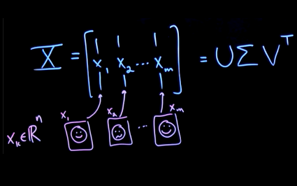
• each column of \(X\) has a face vector \(x_k \in \mathbb{R}^n\)
  • \(n\) is the dimension of our face measurement
• we have \(M\) columns, i.e. different people

SVD allows us to take this matrix \(X\) and decompose/represent it as the product of three other matrices: \(U \Sigma V^T\)

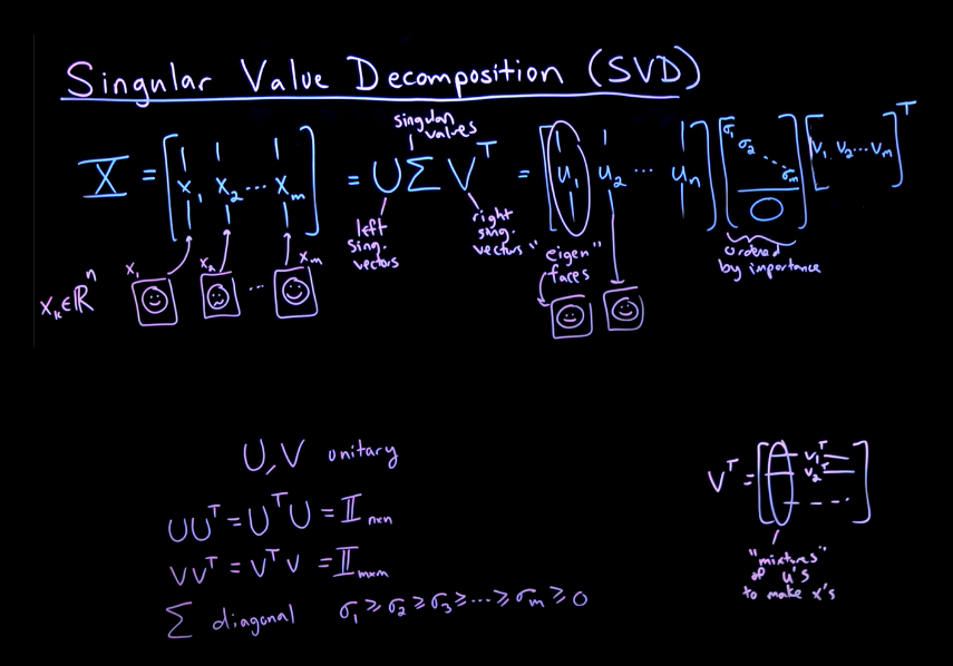
• \(U\) and \(V\) are unitary orthogonal matrices: \(U U^T = U^T U = \mathbb{I}_ {n \times n}\), same with \(V V^T = V^T V = \mathbb{I}_ {m \times m}\)
  • the columns are orthonormal -all orthogonal and have unit length-
• eigen-faces or a column \(U_k\) have the same shape/size as a column of \(X_k\)
  • values of \(u\) are hierarchically arranged according to their ability to describe the variance of the columns of \(X\), the faces
• \(\Sigma\) is a diagonal matrix
  • non-negative and hierarchically ordered (decreasing magnitude): \(\sigma_{m-1} \geq \sigma_m \geq 0\)
  • only \(m\) singular values, the rest is zero
• \(V_k^T\) column tells us the required mixture of \(u\)’s to make \(x\)’s, scaled by the singular value \(\sigma_k\)
  • the first column \(V_1^T\) makes the first column \(X_1\)

interpret \(U\) and \(V\) as eigenvectors of correlation matrices between the rows and columns of \(X\)

We call:

• \(U\) the left singular vector
• \(\Sigma\) matrix of singular values
• \(V\) the right singular vector

Because of the first columns of \(U\), \(\Sigma\) and \(V\) are more important in describing the information of the data matrix \(X\), we can ignore really small singular values \(\sigma\) and approximate the matrix \(X\) only in terms of the first dominant columns of \(U\), \(V\) and \(\Sigma\).

Guaranteed to exist and unique

Matrix Approximation

approximate data matrix X in terms of a lower rank truncated SVD

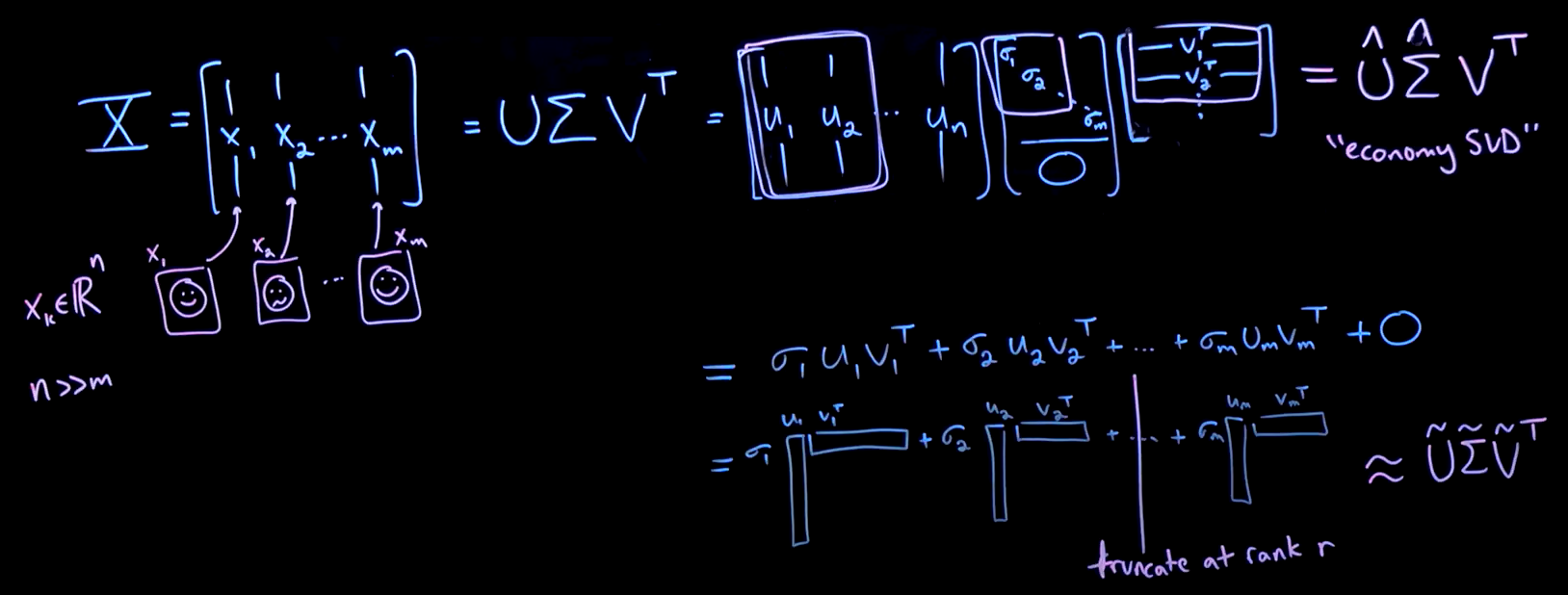Take a data matrix \(X\) and write it as the product of three matrices: \(U, \Sigma, V^T\):

• \(X_{n \times m}\) data matrix at most rank \(M\) due to the columns
  • \(n \gg m\): tall and skinny, e.g. 1_000_000 pixels per column vs 100 people
• \(U_{n \times n}\) contains information about the column space of \(X\)
  • there are only \(M\) nonzero singular values \(\sigma\)
• \(\Sigma_{n \times m}\) weigthing factor of importantance (diagonal matrix)
• \(V^T_{m \times m}\) contains information about the row space of \(X\)

Hierarchically arranged

We can just select as the economy/skinny SVD, i.e. select the non-zero singular values:

• the first \(M\) columns of \(U\) as \(\hat{U}\)
• the first \(M \times M\) block in \(\Sigma\) as \(\hat{\Sigma}\) of nonzero singular values

SVD decomposes the data matrix \(X\) into orthogonal matrices \(U\) and \(V\) that we can rewrite as a sum of these rank one matrices, that increasingly improve the approximation of \(X\). Therefore, we can truncate the summation at rank \(R\), i.e. keep the first \(R\) columns of \(U\), the \(R \times R\) block of \(\Sigma\) and the first \(R\) rows of \(V^T\).

After truncation:

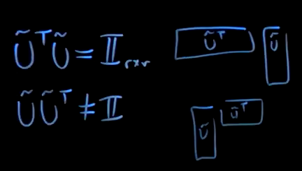
• \(\tilde{U}^T \tilde{U}\) is a \(R \times R\) identity matrix, still orthogonal
• \(\tilde{U} \tilde{U}^T\) no longer the identity matrix after truncation

SVD gives the best low-rank approximation. This is a rank \(R\) approximation of \(X\), i.e. linearly independent columns and rows. Eckart-Young theorem

Dominant Correlations

between the rows/columns of X

\(U\) and \(V\) matrices as eigenvectors of a correlation matrix given by \(X^T X\), every enty is essentially an inner product between two columns of the data matrix \(X\), e.g. correlation between people faces, large value means similar, small means orthogonal different faces:

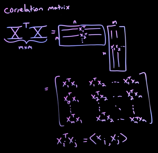
symmetric and positive semi-definite (these are inner products) guarantee to have non negative real eigenvalues that have a direct correspondence on the singular values \(\Sigma\)

The eigenvalue decomposition of the correlation matrix, assuming the economy SVD:

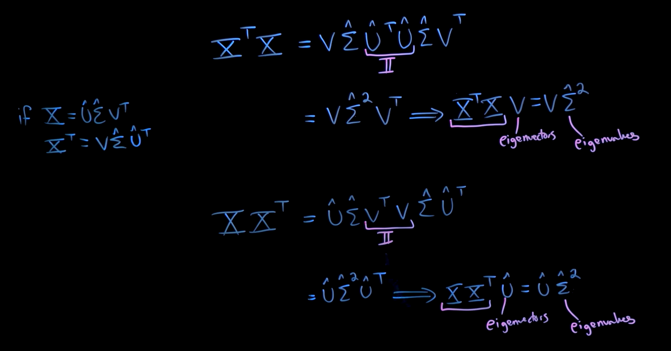
• \(V\): the columns are eigenvectors of the column wise correlation matrix \(X^T X_{m \times m}\)
• \(U\): the columns are eigenvectors of the row wise correlation matrix \(X X^T_{n \times n}\)
• \(\Sigma\): square roots of the eigenvalues of the column/row wise correlation matrix

sorted hierarchically by importantance quantifid by the eigenvalues \(\Sigma^2\)

Methods

Matrix Completion and the Netflix Prize

Very sparse, i.e. values are missing:

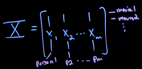
• column: all movie preferences for a person
• rows: different movie

we can use correlations among the columns (people) and correlation among the rows (movies) to discover movie preferences for a given user.

Unitary Transformations

preserve angles and legnths of vectors

Unitary Transformations just rotate our vector space so lengths and angles are preserved.

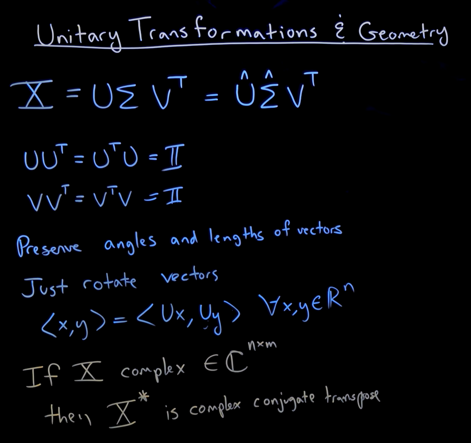
just rotate vectors together

Randomized Singular Value Decomposition

faster efficient SVD for a large data matrix X if we believe it has low intrinsic rank

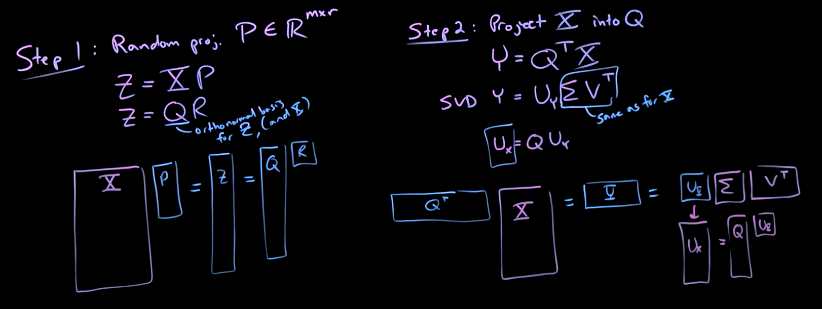
Computing the SVD of a big matrix \(X\) is very expensive but if we believe that there’s a low rank \(r\) structure in there, we can get away with massive reduction computation by first sampling the column space of \(X\) using a a random projection matrix \(P\), then find an orthonormal representation using the QR factorization:

1. compute a random projection \(P\) to multiply with the column space of \(X\) as \(Z = X P\)
   • \(P \in \mathbb{R}^{m \times r}\), \(r\) is the target rank
   • QR factorization as \(Z = Q R\)
   • \(Q\) orthonormal basis for \(Z\) and \(X\)
2. project \(X\) into that low dimensiona subspace \(Q\) as \(Y = Q^T X\), then compute the SVD
   • \(Y = U_r \Sigma V^T\)
   • \(\Sigma V^T\) are the same as the SVD of the original data matrix \(X\)
   • compute \(U_x = Q U_y\)

• oversampling to add more dimensions to \(P\), e.g. \(r + 10\)
• power iterations help when the singular values don’t decay rapidly

Same accurate and efficient representation of the data but in much less computational time.

For larger and/or higher dimensionality datasets there still exists a low intrinsic rank, i.e. key features in the data that actually matter.